"Does vocational training truly boost participants' future earnings?"
For policymakers and business leaders, measuring the real impact of such programs is a critical challenge. A simple comparison between participants and non-participants is often misleading—for instance, highly motivated individuals might be more likely to sign up, skewing the results.
To solve this, we need Causal Inference.
In this post, we revisit a classic case study based on LaLonde's National Supported Work Demonstration (NSW) data. We will move beyond the textbook theory and demonstrate how to strip away bias to uncover the true program effect.
Today, let's analyze this data using Allye Pro.

1. Data Generation
The data is available in the causaldata package. We will use it to create a mixed dataset (nsw_cps_mixed_data) that combines the experimental treatment group with the observational control group.
You can use the code below to generate the data. Or you can also download csv file from here.
from causaldata import nsw_mixtape, cps_mixtape
import pandas as pd
df_nsw = nsw_mixtape.load_pandas().data.copy()
df_cps = cps_mixtape.load_pandas().data.copy()
common_cols = [
"age", "educ", "black", "hisp", "marr",
"nodegree", "re74", "re75", "re78"
]
df_cps_use = df_cps[common_cols].copy()
df_cps_use["treat"] = 0
df_cps_use["source"] = "CPS"
df_nsw_use = df_nsw[df_nsw["treat"] == 1][common_cols + ["treat"]].copy()
df_nsw_use["source"] = "NSW"
df_mixed = pd.concat(
[df_nsw_use, df_cps_use],
axis=0,
ignore_index=True
)
df_mixed['treat'] = df_mixed['treat'].astype('category')
df_mixed.head()
Here is a breakdown of the variables in the dataset:
| Variable | Definition | Role | Details |
|---|
| treat | Treatment Indicator | Treatment | 1 = Received Job Training, 0 = Did not receive. This is the key variable for our analysis. |
| age | Age | Covariate | Age of the participant. |
| educ | Education | Covariate | Years of education completed (e.g., 12 = High School graduate). |
| black | Black (Dummy) | Covariate | 1 = Black, 0 = Otherwise. |
| hisp | Hispanic (Dummy) | Covariate | 1 = Hispanic, 0 = Otherwise. |
| marr | Married (Dummy) | Covariate | 1 = Married, 0 = Single/Other. |
| nodegree | No Degree (Dummy) | Covariate | 1 = No High School Degree, 0 = Has Degree. Used to identify dropouts. |
| re74 | Real Earnings 1974 | Covariate | Pre-treatment Income 1. Indicates economic status before the program. Participants often have low values here. |
| re75 | Real Earnings 1975 | Covariate | Pre-treatment Income 2. Immediate pre-program income. Often zero for participants in this dataset. |
| re78 | Real Earnings 1978 | Outcome | Post-treatment Income. The target variable. We want to see if treat=1 leads to an increase here. |
| source | Data Source | Metadata | Origin of the record ('NSW' for experimental treated, 'CPS' for observational control). |
2. A/A Test and Checking Bias in Treatment Effects
The NSW dataset consists of individuals who sought and received vocational training. The cps_mixtape data, however, represents a general population sample.
There are likely many underlying factors that motivate someone to seek vocational training. First, let's perform a quick A/A Test to check if the two groups are homogeneous.
| Variable | Group | Sample Size | Average | 95% CI | Effect Δ | Lift (%) | p-value | Significant |
|---|
| age | Control | 15992 | 33.23 | [33.05, 33.40] | - | - | - | No |
| Treated | 185 | 25.82 | [24.78, 26.85] | -7.41 | -22.3% | 0.000 | Yes |
| educ | Control | 15992 | 12.03 | [11.98, 12.07] | - | - | - | No |
| Treated | 185 | 10.35 | [10.05, 10.64] | -1.68 | -14.0% | 0.000 | Yes |
| black | Control | 15992 | 0.07 | [0.07, 0.08] | - | - | - | No |
| Treated | 185 | 0.84 | [0.79, 0.90] | +0.77 | +1046.7% | 0.000 | Yes |
| marr | Control | 15992 | 0.71 | [0.70, 0.72] | - | - | - | No |
| Treated | 185 | 0.19 | [0.13, 0.25] | -0.52 | -73.4% | 0.000 | Yes |
| nodegree | Control | 15992 | 0.30 | [0.29, 0.30] | - | - | - | No |
| Treated | 185 | 0.71 | [0.64, 0.77] | +0.41 | +139.4% | 0.000 | Yes |
| re74 | Control | 15992 | 14016.80 | [13868.47, 14165.13] | - | - | - | No |
| Treated | 185 | 2095.57 | [1386.75, 2804.39] | -11921.23 | -85.0% | 0.000 | Yes |
| re75 | Control | 15992 | 13650.80 | [13507.11, 13794.49] | - | - | - | No |
| Treated | 185 | 1532.06 | [1065.09, 1999.02] | -12118.75 | -88.8% | 0.000 | Yes |
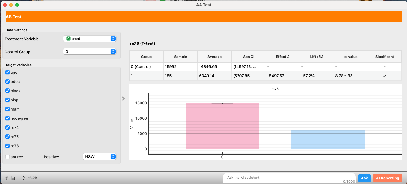
| re78 | Control | 15992 | 14846.66 | [14697.13, 14996.19] | - | - | - | No |
| Treated | 185 | 6349.14 | [5207.95, 7490.34] | -8497.52 | -57.2% | 0.000 | Yes |
Those who received vocational training are generally younger, have lower education levels, and significantly lower pre-training earnings (re74, re75).
Just because the re78 (earnings in 1978) is higher for the non-treated group doesn't mean the training was pointless. It simply suggests that even if the training had a positive effect, it wasn't enough to close the massive initial gap between the two groups. The A/B test reports a negative effect of -$8497.52, but we cannot conclude this is the causal effect of the intervention due to the severe selection bias.
3. Propensity Score Matching
To address this bias, we apply Propensity Score Matching (PSM), a standard technique in causal inference.
We select covariates for balancing (e.g., demographics, prior earnings) and choose the outcome variable.
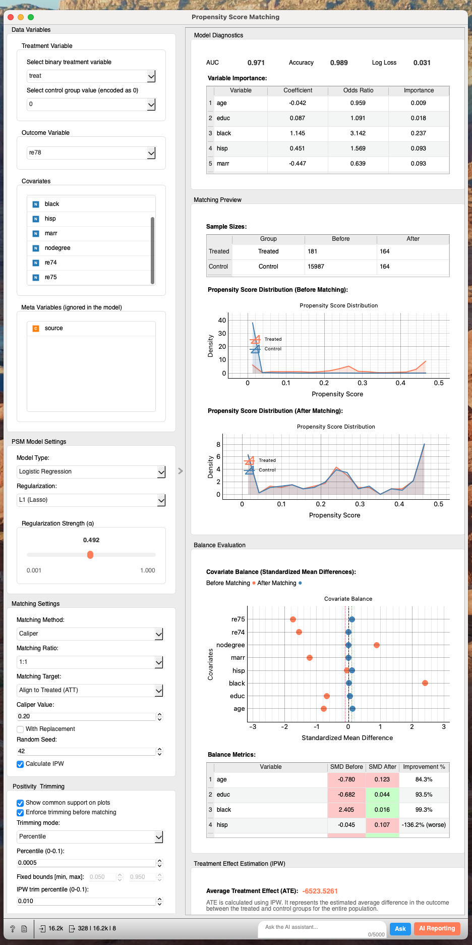
Looking at the Love Plot and the balance table, we can see that the discrepancies identified in the A/A test have been successfully mitigated. The matching process has created a control group that is statistically very similar to the treated group.
Now, let's run an A/B Test on this matched dataset:
| Variable | Group | Sample Size | Average | 95% CI | Effect Δ | Lift (%) | p-value | Significant |
|---|
| re78 | Control (0) | 164 | 4564.52 | [3736.96, 5392.07] | - | - | - | No |
| Treated (1) | 164 | 6429.95 | [5227.35, 7632.55] | +1865.43 | +40.9% | 0.012 | Yes |
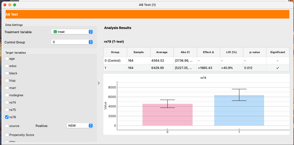
We now estimate a positive effect of $1865.43. This difference is statistically significant.
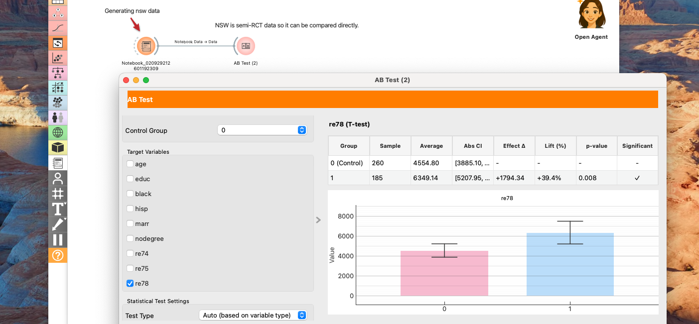
4. Validation: Checking the Answer Key
Since the original NSW dataset is from a Randomized Controlled Trial (RCT), we can calculate the true experimental effect by comparing the treated group with the experimental control group (not the CPS data). (While there is some slight bias in nodegree, the groups are largely balanced.)
Analysis Settings
- Treatment Variable:
treat
- Control Group:
0
- Test Type: Auto (based on variable type)
- Confidence Level: 95%
- Multiple Comparison Correction: None
| Outcome | Group | Sample | Average | Abs CI | Effect Δ | Lift (%) | Effect CI (Δ) | p-value | Significant |
|---|
| age | Control | 260 | 25.05 | [24.19, 25.92] | - | - | - | - | No |
| Treatment | 185 | 25.82 | [24.78, 26.85] | +0.76 | +3.0% | - | 0.266 | No |
| educ | Control | 260 | 10.09 | [9.89, 10.29] | - | - | - | - | No |
| Treatment | 185 | 10.35 | [10.05, 10.64] | +0.26 | +2.6% | - | 0.150 | No |
| black | Control | 260 | 0.83 | [0.78, 0.87] | - | - | - | - | No |
| Treatment | 185 | 0.84 | [0.79, 0.90] | +0.02 | +2.0% | - | 0.647 | No |
| hisp | Control | 260 | 0.11 | [0.07, 0.15] | - | - | - | - | No |
| Treatment | 185 | 0.06 | [0.03, 0.09] | -0.05 | -44.8% | - | 0.064 | No |
| marr | Control | 260 | 0.15 | [0.11, 0.20] | - | - | - | - | No |
| Treatment | 185 | 0.19 | [0.13, 0.25] | +0.04 | +23.0% | - | 0.334 | No |
| nodegree | Control | 260 | 0.83 | [0.79, 0.88] | - | - | - | - | No |
| Treatment | 185 | 0.71 | [0.64, 0.77] | -0.13 | -15.2% | - | 0.002 | Yes |
| re74 | Control | 260 | 2107.03 | [1412.41, 2801.65] | - | - | - | - | No |
| Treatment | 185 | 2095.57 | [1386.75, 2804.39] | -11.45 | -0.5% | - | 0.982 | No |
| re75 | Control | 260 | 1266.91 | [887.97, 1645.85] | - | - | - | - | No |
| Treatment | 185 | 1532.06 | [1065.09, 1999.02] | +265.15 | +20.9% | - | 0.385 | No |
| re78 | Control | 260 | 4554.80 | [3885.10, 5224.50] | - | - | - | - | No |
| Treatment | 185 | 6349.14 | [5207.95, 7490.34] | +1794.34 | +39.4% | - | 0.008 | Yes |
The true effect is +$1794.34. Our PSM estimate of $1865.43 differs by less than 4%, demonstrating that PSM was able to recover the causal effect with high accuracy from the observational data.
5. Advanced Topics: Heterogeneous Treatment Effects
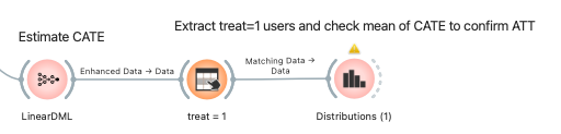
Using machine learning, we can go a step further and estimate the Conditional Average Treatment Effect (CATE) for individuals. Given the small sample size and high variance, we'll use LinearDML, which provides robust CATE estimation.

By averaging the predicted CATE for the treated individuals (treat = 1), we can compare this result with our previous average treatment effects.
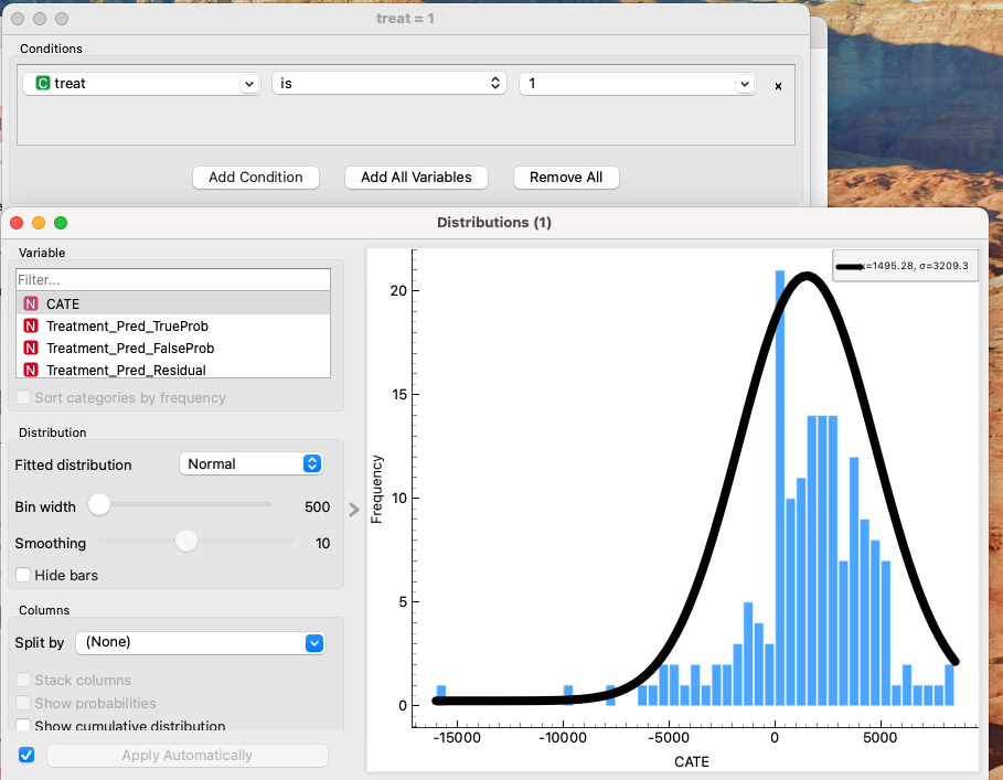
The calculated result is $1495. While there is a ~16.7% deviation from the true $1794, it is a massive improvement over the naive observational comparison (-$8497) and provides a directional estimate good enough for decision-making.
One more tip for the accurate understanding
In the LinearDML report, the factors contributing to CATE showed that both re74 and re75 had negative coefficients, with re74 showing a particularly strong negative correlation.
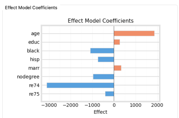
It makes intuitive sense that people with higher prior earnings might benefit less from basic vocational training. However, the fact that re74 (income 4 years prior) had a much stronger correlation than re75 (income 3 years prior) seemed odd.
Before jumping to conclusions, we should check for multicollinearity, as LinearDML (being a linear model) is sensitive to it.
Checking the scatter plot and correlation between re74 and re75, we find a high correlation coefficient (r=0.87). The plot also suggests a ceiling effect.
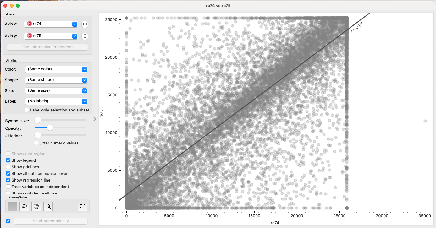
This collinearity might be distorting the coefficients. To fix this, we can filter out the ceiling values as outliers and apply Principal Component Analysis (PCA) to re74 and re75 to create orthogonal components.
- PC1: Positively correlated with both
re74 and re75 (represents overall income level).
- PC2: Represents the difference/variance between the years.
Re-running LinearDML with PC1 and PC2 instead of the raw variables yields the following:
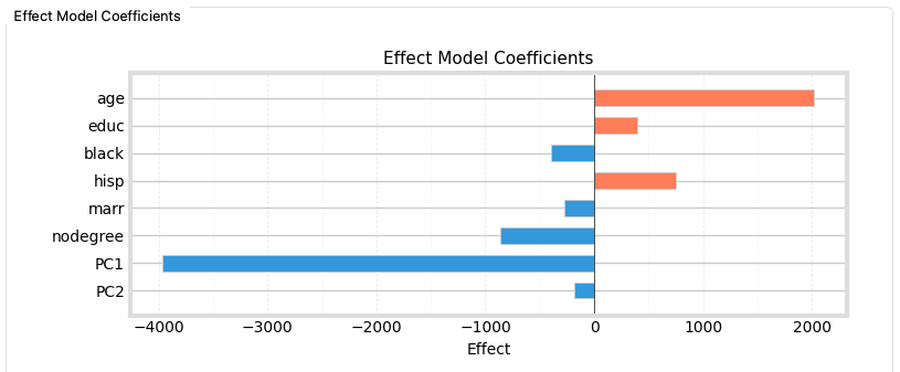
Both components still show a negative correlation with CATE, but PC1 (overall income level) has the strongest negative correlation. This confirms our hypothesis: Vocational training is less effective for those who already have high earning potential. It wasn't about re74 specifically, but the general income level.
Additionally, age shows a positive correlation, suggesting that older participants (within this demographic) benefited more from the training than younger ones.
6. Conclusion and Summary
Our analysis of the NSW vocational training program revealed several key insights:
- Bias Correction: Simple comparison of observational data led to a misleading negative effect (-$8500). Propensity Score Matching successfully corrected this bias, estimating a positive effect (+$1865) very close to the true experimental benchmark (+$1794).
- Targeting Efficiency: Vocational training budgets and manpower are limited. To maximize effectiveness, our CATE analysis suggests a clear policy direction:
- Focus on those with lower prior earnings. The training has diminishing returns for those with higher baseline income.
- Prioritize older applicants. Within this group, older individuals showed higher treatment effects.
Simply looking at post-training income (re78) might tempt administrators to select candidates who are likely to earn more anyway (high prior earners). However, our causal analysis proves this would be a mistake—those individuals benefit the least from the program. The true value of the training is maximized by targeting those who need it most.
Data Science Is Fun! Getting It Right Is What Makes It Valuable.
Achieve deeper understanding and higher-quality outputs in data science—beyond your peers.
If you want to explore the data yourself, grab the dataset and try reproducing these results in Allye!
You can try Allye Base for free.

